PoTM - Understanding Dataset Difficulty with V-Usable Information
In this post, I would like to summarize an interesting paper that received the Outstanding Paper Award at ICML 2022: Understanding Dataset Difficulty with V-Usable Information (Ethayarajh et al.). The paper introduces a novel method for estimating the difficulty of a dataset w.r.t. a model using information theory. Specifically, it proposes \(\mathcal{V}\) - usable information and pointwise \(\mathcal{V}\) - usable information extended from Shannon’s mutual information to measure how much information contained in a dataset \((X, Y)\) (\(X\): input, \(Y\): label for example) or in an instance of \((X, Y)\) is usable by a model \(\mathcal{V}\). Lower value \(\mathcal{V}\) - usable information indicates that the dataset (or the instance) is more difficult for the model \(\mathcal{V}\).
Table of Contents
- The lack of interpretability for estimating dataset difficulty of related works
- Shannon Mutual Information
- \(\mathcal{V}-usable\) information (or \(\mathcal{V}\) information)
- Pointwise \(\mathcal{V}\) information
- Usage of \(\mathcal{V}\) information
The lack of interpretability for estimating dataset difficulty of related works
-
Typical strategy of assessing whether a dataset is hard is to benchmark state-of-the-art models on this dataset and compare their performances to human. The bigger gap, the harder the data is considered to be. Since such evaluation is generally done at dataset-scale, it is limited in the capacity of understanding the different difficulty of individual sample in the dataset (which sample is harder than other). Furthermore, classic performance metrics, such as accuracy or F1 score for classification problem, are not suitable for standardized comparison across models and datasets. For example, considering 2 datasets \((X_1, Y_1)\) and \((X_2, Y_2)\) where \(X_1\) (resp. \(X_2\)) is independent of \(Y_1\) (resp. \(Y_2\)), we should expect that they have the same highest level difficulty (\(\mathcal{V}\) - usable information \(\approx\) zero), however, a model can obtain different accuracy on two datasets depending on the frequency of the majority class \(y\) in the dataset.
-
Model-agnostic approaches to estimate the difficulty of a dataset are not able to explain why the dataset is easy for some models and hard for other models.
-
Some approaches consider text-based heuristics such as word identity, input length or learning-based metrics such as training loss, prediction variance as proxies for dataset difficulty. However, they are not as readable as \(\mathcal{V}\) - usable information.
Shannon Mutual Information
Shannon mutual information between two random variables measures the the amount of information obtained about one random variable (or the change in entropy of one random variable) by observing the other random variable (in the context of dataset difficulty, \(X\) is the input variable and \(Y\) is the label variable):
\[I(X, Y) = H(Y) - H(Y \mid X)\]However, because this quantity is calculated with the assumption of infinite computation capacity, it is not suitable in practice as computational constraint is an important aspect to be considered. For example, considering three datasets \((X, Y)\), \((f(X), Y)\) and \((g(X), Y)\) where \(f\), \(g\) is an encrypting function and an useful preprocessing function applied on \(X\), respectively, we should expect that using \(f(X)\) to predict \(Y\): \(f(X) \rightarrow Y\) is harder and using \(g(X)\) to predict \(Y\): \(g(X) \rightarrow Y\) is easier than using \(X\) to predict \(Y\): \(X \rightarrow Y\) as after encrypting \(X\), the information contained in \(X\) becomes less accessible or after pre-processing \(X\), the information contained in \(X\) is exploited more easily. Despite that, the Shannon mutual information \(I(X, Y)\) would not change: \(I(X, Y) = I(f(X), Y) = I(g(x), Y)\) as it allows for unbounded computation, so one can employ arbitrarily complex strategy to decode \(f(X)\) and predict \(Y\) from \(X\).
\(\mathcal{V}-usable\) information (or \(\mathcal{V}\) information)
Let \(\mathcal{X}, \mathcal{Y}\) be the sample space of two random variables \(X\), \(Y\) respectively and \(\Omega = \{f: \mathcal{X} \cup \varnothing \rightarrow \mathcal{P}(\mathcal{Y}) \}\) be any mapping function that predicts a distribution over \(\mathcal{Y}\) using the input \(\mathcal{X}\) or no side information \(\varnothing\). The computation-unbounded Shannon mutual information can be rewritten as: \(I(X, Y)=I_{\Omega}(X, Y)\).
Under the computational or statistical constraints scenario, only a subset \(\mathcal{V} \subset \Omega\) is allowed to use to predict \(Y\), leading to the definition of \(\mathcal{V}\) information, extended from Shannon mutual information:
\[I_{\mathcal{V}}(X, Y) = H_{\mathcal{V}}(Y) - H_{\mathcal{V}}(Y \mid X)\]where \(H_{\mathcal{V}}(Y) = \inf_{f \in \mathcal{V}} \mathbb{E}_{y \sim Y}[-\text{log} \; f[\varnothing](y)]\) and \(H_{\mathcal{V}}(Y \mid X) = \inf_{f \in \mathcal{V}} \mathbb{E}_{y \sim Y, x \sim X}[-\text{log} \; f[x](y)]\).
Intuitively, the conditional \(\mathcal{V}-entropy\) \(H_{\mathcal{V}}(Y \mid X )\) (resp. \(\mathcal{V}-entropy\) \(H_{\mathcal{V}}(Y)\)) is smallest expected negative log-likelihood of predicted label \(Y\) given observations \(X\) (resp. no side information \(\varnothing\)).
In practice, it is impossible to calculate the true \(\mathcal{V}-information\) as it requires the whole data distribution. Instead, it is empirically estimated on a finite dataset supposed to include samples that i.i.d drawn from the distribution, leading to the gap between the true \(\mathcal{V}-information\) and empirical \(\mathcal{V}-information\). However, if \(\mathcal{V}\) is less complex and the dataset is large, the gap becomes small.
In the learning context, \(H_{\mathcal{V}}(Y \mid X )\) is estimated by training (or fine-tuning) a model \(f \in \mathcal{V}\) with cross-entropy loss to minimize the negative log-likelihood of \(Y\) given \(X\): \(\mathbb{E}_{y \sim Y_{train}, x \sim X_{train}}[-\text{log} \; f[x](y)]\), then using the trained model to calculate \(\mathbb{E}_{y \sim Y_{test}, x \sim X_{test}}[-\text{log} \; f[x](y)]\) on test dataset. Similarly, \(H_{\mathcal{V}}(Y)\) is estimated by fitting another model \(f \in \mathcal{V}\) on label distribution.
Pointwise \(\mathcal{V}\) information
\(\mathcal{V}\) information is extended to individual instance \((x, y)\) of random variables \((X, Y)\) under pointwise \(\mathcal{V}\) information \(\textsf{PVI}(x, y)\).
\[\textsf{PVI}(x \rightarrow y) = - \text{log} \; g[\varnothing](y) + \text{log} \; g'[x](y)\]where \(g \in \mathcal{V} \; s.t. \mathbb{E}[- \text{log} \; g[\varnothing](Y)] = H_{\mathcal{V}}(Y)\) and \(g' \in \mathcal{V} \; s.t. \mathbb{E}[- \text{log} \; g'[X](Y)] = H_{\mathcal{V}}(Y \mid X)\). Loosely speaking, \(g\) and \(g'\) are models (e.g. BERT) before and after fine-tuning with training samples of \((X, Y)\), and \(\textsf{PVI}(x, y)\) is the difference in log-probability that two models assign to the label \(y\). The higher the \(\textsf{PVI}\), the easier the instance is w.r.t. \(\mathcal{V}\).
\(\textsf{PVI}(x, y)\) should only depend on the distribution of \(X\) and \(Y\). Fine-tuning models \(\in \mathcal{V}\) with different size of training set \(\{(x, y)_i\}_{i=1}^k\) should not change this quantity.
The estimated \(\mathcal{V}\) information \(\hat{I}_{\mathcal{V}}(X, Y)\) is written as: \(\hat{I}_{\mathcal{V}}(X, Y) = \frac{\sum_i \text{PVI} (x_i, y_i)}{n}.\)
Usage of \(\mathcal{V}\) information
-
Compare different models \(\mathcal{V}\) for the same dataset \((X, Y)\) by computing \(I_{\mathcal{V}}(X \rightarrow Y)\)
Following figure shows the test accuracy of 4 models {GPT2-small, BERT-base, BART-base, DistillBERT-base } on SNLI task. Model with higher \(\mathcal{V}-information\) exploits more information from the dataset, leading to better performance (BART-base).
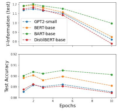 (Source: copied from the paper)
Furthermore, \(\mathcal{V}-information\) can be an early sign of overfitting. At epoch 5, the models start to be less certain about the true label \(\rightarrow\) \(\mathcal{V}-information\) starts to decrease but it can still make correct predictions (test accuracy is stable). Then, at epoch 10, \(\mathcal{V}-information\) reach its lowest value and diverges but it looks like test accuracy is just starting to decline.
-
Compare the difficulty of different dataset \((X, Y)\)(s) for the same model \(\mathcal{V}\) by computing \(I_{\mathcal{V}}(X \rightarrow Y)\)
The dotted lines in figure below show \(BERT-information\)(s) (\(\mathcal{V}\) = BERT) for 3 NLI datasets: CoLA, MultiNLI and SNLI. It is expected that CoLA is the most difficult dataset, then MultiNLI for NLI task addressed by BERT model.
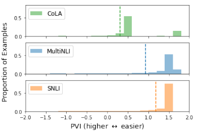 (Source: copied from the paper)
 -
\(\textsf{PVI}\) can help to spot mislabelled instances where such instances have negative \(\textsf{PVI}\).
-
The \(\textsf{PVI}\) threshold at which predictions become incorrect is similar across datasets. The gold threshold is 0.5 which is useful for cross-dataset comparison.